Blog Article & Copyright by Lukas Hillesheim
The first article of this series is intended to explain the complex language DAX from the point of view of other concepts, on the internet the term projection is often used for this. Other concepts can be set concepts, OOP concepts and concepts from SQL. Concepts from other languages can make DAX more transparent.
1. DAX as a language for End Users
SelfService. When delivering DAX to the developers community, the idea of SelfService was emphasized. Therefore, the usability of BI products is aligned to the need of power users, not to BI professionals. Complexity is hidden from the DAX developer as much as possible and many standard behaviors of the DAX language and the Power BI product ensure compact code and a fast path to the solution.
Complexity. The fact that DAX is a really complex language is therefore not apparent to the beginning DAX developer. The fact of complexity and its reasons was therefore worth its own article.
My series is intended to make DAX more transparent by the help of other concepts:
- - Set concepts. Objects such as SETs, TUPELs, MEMBERs
- - Operations like CROSSJOIN, INTERSECT, EXCEPT
- - SQL-Code
- - OOP-Pseudo-Code
Set concepts and tupels. If you keep in mind that MDX and DAX work as sibling languages on the same backend, the Vertipaq engine, it is obvious that the way from MDX to DAX and vice versa is very short: MDX with its sets, tuples and members can be thought as the native language for the dimensional backend. So with every line of DAX code, you can also ask yourself which set operations actually take place in the background.
The series fokuses on users who have already some experiences with DAX and are familiar with the concepts of Filter, Context Transition und Filter Propagation introduced by Marco Russo and Alberto Ferrari. Knowledge of SQL and / or an object-oriented language such as C# is also advantageous.
2. Basic Operation CrossJoin in the DAX function CROSSJOIN
The idea of CROSSJOIN is to apply each member of set 1 to each member of set 2. The example shows the CROSSJOIN for two 1-dimensional tuple sets. Set 1 contains letters, set 2 contains numbers. The result of the link is a 2-dimensional tuple set. A set is syntactically represented with "{}" and a tuple with "()".
- set1 = { A, B }
- set3 = set1 CROSSJOIN set2
- Inhalt von set3: { (A, 1 ), (A, 2), (A, 3), (B, 1), (B, 2), (B, 3) }
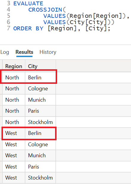
DAX-Example / CROSSJOIN-Function.
The DAX function CROSSJOIN behaves as expected in theory and shown above. It computes the complete cartesian product of region and city.
3. Basic CrossJoin operation in the DAX function SUMMARIZECOLUMNS
Syntax of SUMMARIZECOLUMNS:
- SUMMARIZECOLUMNS (
- <groupBy_columnName> [, < groupBy_columnName >]…,
- [<filterTable>]…
- [, <name>, <expression>]…)
Only the first argument type is mandatory: one or more grouping columns must be specified. The next example shows the use of SUMMARIZECOLUMNS with the corresponding sample data from above. Only the first mandatory argument type is used:
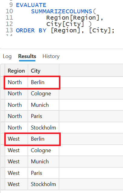
DAX-Example / SUMMARIZECOLUMNS on a Snowflake-Schema.
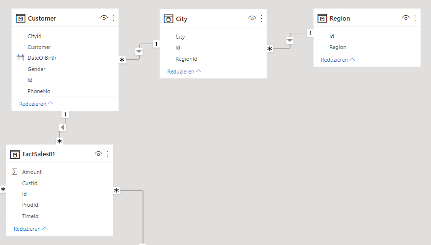
The example proves that the main operation of SUMMARIZECOLUMNS is actually a CROSSJOIN using the groupby columns. In the example, the data model behind the DAX query is a snowflake schema. The entities City and Region are stored in separate tables and connected via relationships:
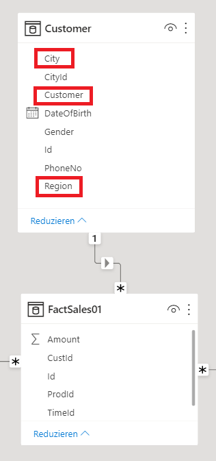
DAX example / SUMMARIZECOLUMNS on a star schema. The next example shows another query with SUMMARIZECOLUMNS and the same data. However, the Region and City entities are available through a table holding that data in a denormalized form. The undelying model is based on a star scheme:
The DAX query now produces a different result:
The complete cross matrix was no longer returned; Berlin for example only occurs together with the North.
Rules:
The CROSSJOIN function returns the complete cross matrix – regardless of the data model
Basically the SUMMARIZECOLUMNS function performs an CROSSJOIN too, but optionally restricts the result to existing ones. The restriction depends on the table where the columns reside.
SUMMARIZECOLUMNS / Steps:
1. Compute the complete cross matrix
2. Optional: Restrict the tuple set
4. SQL Example / Projection of SUMMARIZECOLUMNS
The following two examples show the set operations as they can be thought of in SQL.
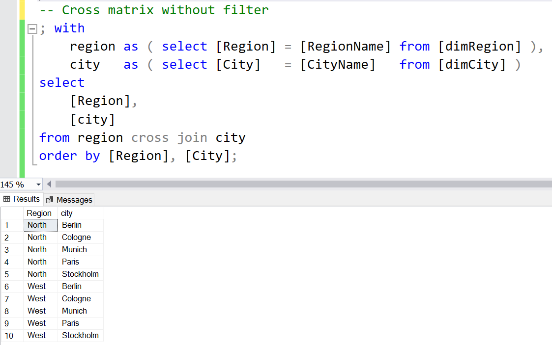
SQL example / return a complete cross-matrix without filters. The column values come from two different tables:
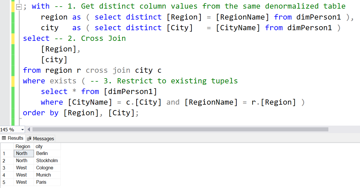
SQL example / return of a complete cross-matrix with filter. Note the following difference from the previous example: The values for Region and City are now both from the same table [dimPerson1]. After the complete cross matrix has been computed, the table [dimPerson1] is used to return only the tuples that actually exist.
The general takeaway from the second example is that tables provide a list of valid tuples that can be used to filter other sets.
