Blog Article & Copyright by Lukas Hillesheim
Series, such as time series, are useful when it comes to making predictions or recognizing patterns. KQL offers a bunch of features for working with series. The following article shows how make-series and series-fill-linear may help you in deriving missing values from the existing ones based on interpolation.
Content:
- 1. Scenario
- 2. Complete KQL code
- 3. Series without gaps | Visualization
- 4. Series with gaps
- 5. Reconstruct missing items
- 6. Reconstruct missing values
- 7. Visualization as linechart
1. Scenario
Underlying scenario for this blog article:
- Step 1. Generate a series that represents a sinusoid and assign the series to a variable
- Step 2. A range from 0.5 to 1 is removed from the series and applied to a variable called missing_range
- Step 3. Based on missing_range a new series is derived and assigned to a variable named recomp_xitems. recomp_xitems contains new, artificially generated items that represent the x-axis items of the sinusoid. Each of the new items has a default value of -1
- Step 4. A new series is computed and applied to the variable recomp_yitems. The default value -1 is replaced with a new value that fits into the sinusoid.
2. Complete KQL code
Complete KQL code for this article. Each code block will be explained separately:
let sinusoid =
    print x = range(0.01, 5, 0.03)
    | mv-expand x
    | serialize
    | extend
        row_ix = row_number(1),
        x = round(todouble(x), 2),
        y = sin(todouble(x))
    | project-reorder
        row_ix,
        x,
        y
    | sort by row_ix asc;
let missing_range =
    sinusoid
    | where x < 0.5 or x > 1;
let recomp_xitems =
    missing_range
    | make-series
        y = avg (todouble(y))
        default = -1 // Set -1 for new items
        on x
        from 0.1 to 5
        step 0.03;
let recomp_yitems =
    recomp_xitems
    | extend
        y = series_fill_linear(y, -1, false);
recomp_yitems
    | mv-expand x, y
    | serialize
    | extend
        row_ix = row_number(1),
        x = round(todouble(x), 2),
        y = todouble(y)
    | render linechart with (xcolumn=x, ycolumns=y)
3. Series without gaps | Visualization
The following KQL code block shows how the sinusoid series is computed and visualized:
- The series is based on a decimal array (lower bound = 0.01, upper bound = 5) that is generated by the KQL function range. The increment of 0.03 is responsible to avoid any artifacts.
- A column named row_ix with an auto id is added as row identifier.
- At least the series is applied to the sinusoid variable and visualized by render
KQL code:
let sinusoid =
    print x = range(0.01, 5, 0.03)
    | mv-expand x
    | serialize
    | extend
        row_ix = row_number(1),
        x = round(todouble(x), 2),
        y = sin(todouble(x))
    | project-reorder
        row_ix,
        x,
        y
    | sort by row_ix asc;
sinusoid
| render linechart with (xcolumn=x,ycolumns=y)
Output:
4. Series with gaps
The KQL code of section 4 simulates a common situation where data is missing. The series contained in the variable sinusoid is modified and the range between 0.5 and 1 is removed from the series. The result is applied to the variable missing_range:
KQL code:
let missing_range =
    sinusoid
    | where x < 0.5 or x > 1;
missing_range
Output:
5. Reconstruct missing items
In the next step the KQL function make-series is applied to the missing_range series thereby computing new items with a default value of -1.
KQL code:
...
let recomp_xitems =
    missing_range
    | make-series
        y = avg (todouble(y))
        default = -1 // Set -1 for new items
        on x
        from 0.1 to 5
        step 0.03;
recomp_xitems
Output:
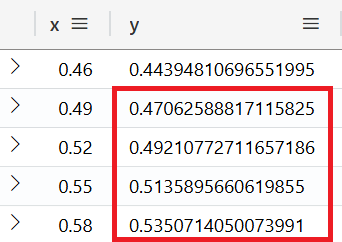
The screenshot above shows that the x-/y-axis tupel members reside separated from each other in two arrays. In order to extract a list of tupels from the two arrays, both arrays must be crossed simultaneously. E.g. x[0] and y[0] form the tuple (0.1, 0.0998334). In Python a function named map is able to do this, in KQL a similiar function named mv-expand exists. In order to understand, how make-series is going to add new items, the next code block presents the content of both arrays as a 2-column table. This separate step is dedicated to educational purpose only and is not part of the complete KQL code mentioned above. The array expansion would be superfluous because in the next step series-fill-linear requires the data in an array layout.
The output is restricted to x-items greater or equal 0.46.
The output is restricted to x-items greater or equal 0.46.
KQL code:
...
let recomp_xitems =
    missing_range
    | make-series
        y = avg (todouble(y))
        default = -1 // Set -1 for new items
        on x
        from 0.1 to 5
        step 0.03;
recomp_xitems
    | mv-expand x, y
    | extend
        x = round(todouble(x), 2)
    | project-reorder
        x,
        y
    | where x >= 0.46
    | sort by x asc
Output:
6. Reconstruct missing values
In the last step the KQL function series-fill-linear replaces the dummy values -1 with new values that fit into the sinusoid. This is done using interpolation.
KQL code:
...
let recomp_yitems =
    recomp_xitems
    | extend
        y = series_fill_linear(y, -1, false);
recomp_yitems
Output:
Similar to 5. Reconstruct missing items, the arrays are unzipped in order to present their content:
KQL code:
...
let recomp_yitems =
    recomp_xitems
    | extend
        y = series_fill_linear(y, -1, false);
recomp_yitems
    | mv-expand x, y
    | extend
        x = round(todouble(x), 2)
    | project-reorder
        x,
        y
    | where x >= 0.46
    | sort by x asc
Output:
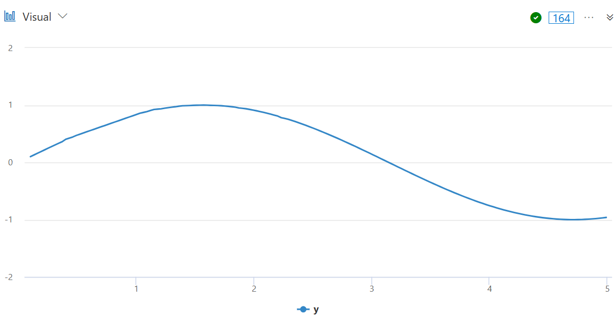
7. Visualization as linechart
The now reconstructed series is presented through a linechart.
KQL code:
...
recomp_yitems
    | mv-expand x, y
    | serialize
    | extend
        row_ix = row_number(1),
        x = round(todouble(x), 2),
        y = todouble(y)
    | render linechart with (xcolumn=x, ycolumns=y)
Output:
Especially the reconstructed area from 0.5 to 1 is not so smooth as the rest of the linechart. Optimization features could help in order to remove the artifacts.


