Attribute relationships are internal objects of the Analysis Services MultiDimensional Engine. They are not visible for the MDX client, can only be used indirectly and can only be configured in the development environment. However, they affect MDX objects and implicit behaviors. Understanding relationships is therefore essential for understanding MDX.

Attributes are the building blocks within Analysis Services MultiDimensional. Attributes are used to derive attribute hierarchies, hierarchies with multiple levels and element properties. They also control implicit behaviors such as MDX [<hierarchy>].CurrentMember and AutoExist.

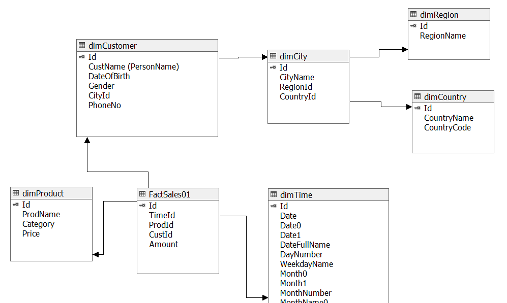
The examples of this document use the following data model:

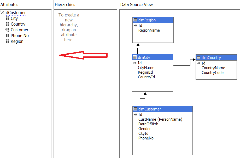
Extraction of SSAS attributes from SQL table columns. SSAS MultiDimensional makes the contents of table columns available though attributes. Mapping of attributes on table columns is configured in SSDT:

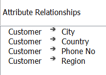
In the example, there is a key attribute [Customer] that get it´s data from the table column [dimCustomer].[Id]. The attribute - which originally has the same name as the column - was renamed to [Customer]. In addition, there are various non-key attributes [City], [Country], [Region] and [Phone No]. By default, all attributes have a direct relationship to the key attribute:

Please note that there are two types of relationships: 1. relationships in SSAS between attributes and 2. relationships between tables in the relational model. Only attribute relationships are relevant for understanding MDX.

Please also note, that in terms of relationships, there is a fundamental difference between SSAS MultiDimensional and SSAS Tabular. In a tabular environment, relationships between tables are presented to the DAX client and must be considered as part of the DAX language.

The SSAS MultiDimensional engine exports the following objects types:

The distinction between "Attribute Hierarchy" and "MultiLevel Hierarchy" is part of this article and it is import for the general understanding, but the distinction between both types is not relevant from a syntactic point of view.

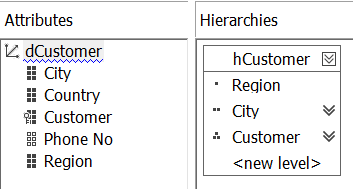
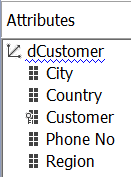
Without further intervention, each attribute is exported as a hierarchy. List of attributes:

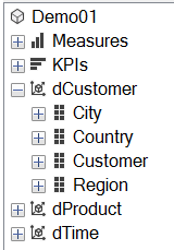
List of hierarchies of the [dCustomer] dimension:

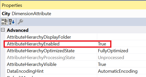
This default behavior is set through the attribute's "AttributeHierarchyEnabled" property. [City] attribute properties:

If "AttributeHierarchyEnabled" is set to "true", aggregation is applied to each member. E.g. for the members [Berlin], [Madrid] etc. [Sum] and [Count] are computed and added to the cube data. In addition, the artificial member [ALL] is created and also added to the hierarchy. The value of [ALL] derives from the "aggregate of the aggregates".

Some data is not interesting in the sense of aggregation, but in the sense of description. This applies, for example, to the [Phone No] attribute. It does not make sense to compute aggregates according to telephone numbers, but it is useful to display the telephone number along with a customer.

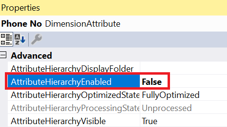
Disabling "AttributeHierarchyEnabled" makes the attribute disappear from the list of hierarchies, but the data of the attribute is still part of the cube and can be used in other ways (see below):

[Phone No] is still part of the attribute list; but is assigned a different icon:

[Phone No] is no longer part of the hierarchy list:

Attribute relationships turn an attribute on the right side of a relationship into a property of the attribute on the left.

Switching "AttributeHierarchyEnabled" off has no affected on the relationships mentioned above. [Phone No] is still on the right side and [Customer] on the left side of an attribute relationship. In other words, [Phone No] is still a member property of [Customer]. This fact is expressed by the following MDX code:

Since [City], [Region], and [Country] are also related to [Customer] - each residing on the right side of an attribute relationship - they all are properties of [Customer]:

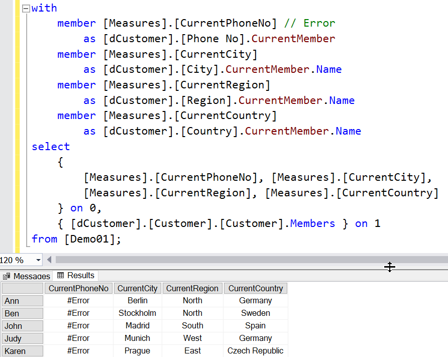
Another effect of attribute relationship is that member selection on one side of the relationship implicitly controls the CurrentMember on the other side. This works from left to right and vice versa. For example, while [Customer].[John] is selected on the left side, [City].CurrentMember on the right side is automatically set to [City].[Madrid]. If - on the other hand - [City].[Madrid] was selected on the right side, [Customer].CurrentMember was implicitly set to [Customer].[All]. Please additionally note, that accessing [Phone No].CurrentMember causes an error because the CurrentMember function can only be applied to hierarchies: [<hierarchy>].CurrentMember.

Example where the attribute relationships works from left to right:

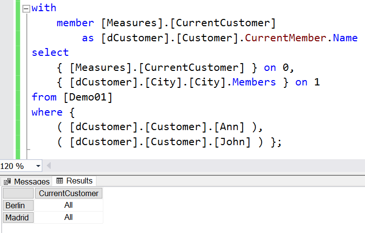
The following example shows how the attribute relationship works from the right to the left side. Members from the [City] hierarchy are iterated over using the expression "[dCustomer].[City].[City].Members". While the iteration takes place, the Measure-Expression "[dCustomer].[Customer].CurrentMember" is evaluated. Because [Customer].CurrentMember is implicitly driven by the right side, it is set to [Customer].[All] thereby overriding the Slicer Axis! The Slicer Axis initially sets a context for the iteration with a restriction to [Ann] and [John]. Due to the restriction - placed on the left side (!) - only those cities where [Ann] and [John] live - are selected for the iteration. This explains, why only two cities are visible. During the iteration, the Initial Context from the Slicer Axis including [Ann] and [John] is overridden with a new Runtime Context which sets [Customer].CurrentMember constantly to [Customer].[ALL]. This example demonstrates the effect of attribute relationships twice!

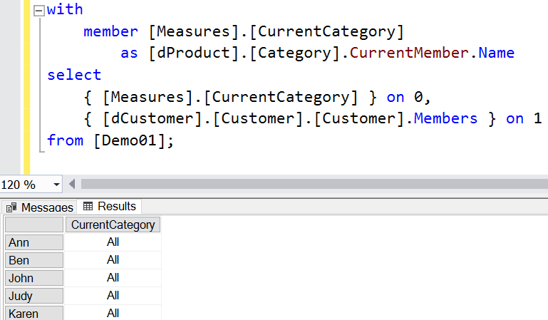
There are no relationship between attributes of the [dCustomer] dimension and attributes of the [dProduct] dimension. Attribute relationships end at the boundary of a dimension. In the absence of a relationship between [Customer] and [Category], [Category].CurrentMember cannot be modified and remains constantly [ALL]:

The data stored in the attributes of a dimension can express hierarchical facts. For example, customers are located in a specific city, which in turn is located in a specific region. Viewed from above, the result is a tree – with [ALL] at the top level, a 2nd level with regions, a 3rd level with cities and a 4th level with customers.

In the Dimension Editor, a developer can create hierarchies with multiple levels from hierarchy-enabled attributes. The example shows how the hierarchy [hCustomer] is derived from [Region], [City], and [Customer]:

For the hierarchy to "work", there are two conditions to match:

1. Attribute relationships should be defined to express the parent-child relationship between the respective entities. This means that the lower level should have an N:1 relationship to the higher level. Without this relationship, there are either schema errors or potential performance issues.

2. The data must satisfy the relationships. For example, a relationship defined as N:1 requires [City].[Madrid] to have only a single combination with [Region]; that´s [Region].[South]. If another combination of [City].[Madrid] with another region such as [North] was found when processing the dimension, the cube would abort the process with errors.

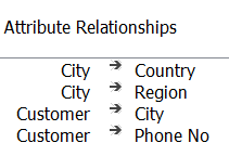
Relationships for the example:

Transitive Relationships. The change in the relationship model results in additional behaviors that you should be aware of: Attribute relationships are transitive / cascading. For example, with [Customer].[John] on the left side of the relationship "Customer -> City", not only [City].CurrentMember is set to [City].[Madrid], but the cascading nature of the relationships additionally sets [Region].CurrentMember to [Region].[South] and [Country].CurrentMember to [County].[Spain].

Members as pointers. The multi-level hierarchy technically represents a bunch of pointers to the underlying attributes. The member [John] from the [hCustomer] hierarchy is essentially a pointer to the member [John] from the hierarchy [Customer]. In the background, the relationships provide a kind of "pointer synchronization".

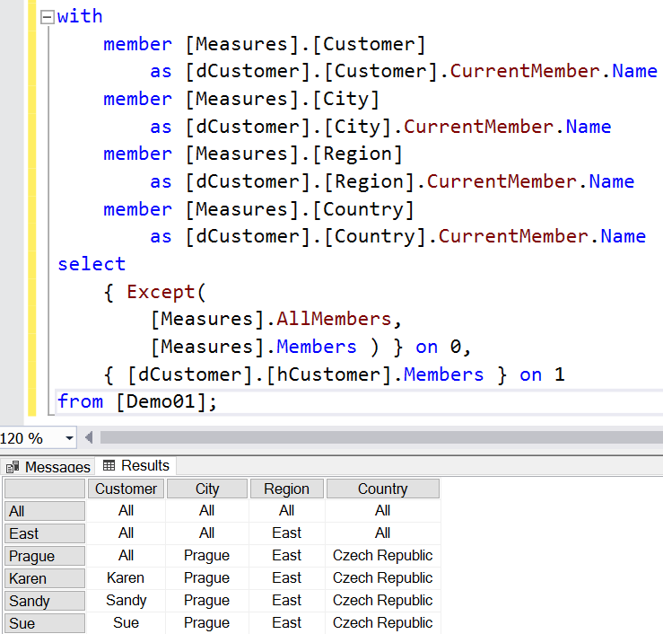
The following example shows an iteration over the members of [hCustomer]. As an affect of the underlying attribute relationships, each CurrentMember of each participating hierarchy is modified. The iteration on [hCustomer] regards all members of the hierarchy on their respective levels including the top level. For members at the "Customer" level, the grids shows a complete "information" according to [City], [Region] and [Country]. The members of this level such as [Karen] are located on the left side of the "leftmost" relationship. Transitivity reaches all hierarchies and their right-hand CurrentMembers. For members of the "City" level such as [Prague] there is an incomplete "information"; [Customer].CurrentMember is set to [ALL]. This is because [City] is on the right side of the relationship and [Customer] is on the left.

From a user´s point of view, the question of whether a particular tuple "exists" can be defined in two ways:

 

 

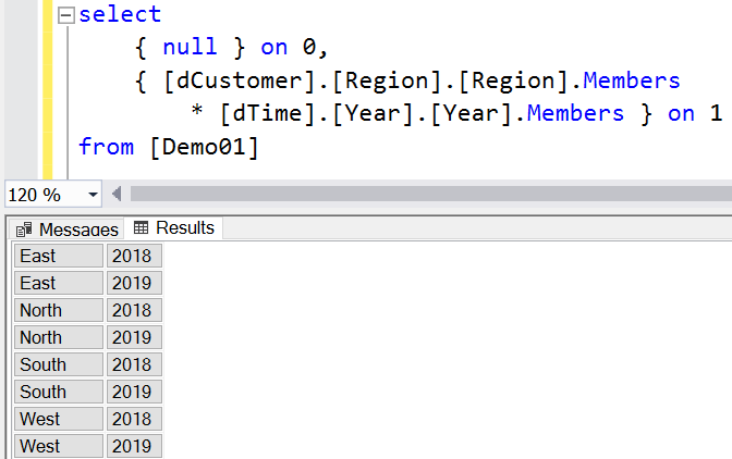
Here are two examples. The first example crossjoins [Region] and [Year]. Because both hierarchies are in different dimensions, AutoExist cannot impose a restriction.

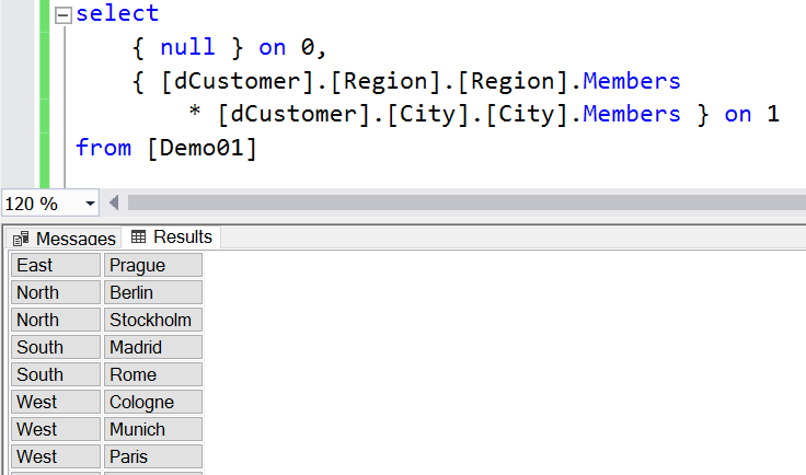
In the second example, a CrossJoin is performed between [Region] and [City]. In this case, AutoExist has a restrictive effect.

Example 1: [Region] CrossJoin [Year]. The complete Cartesian Product is formed.

Example 2. [Region] CrossJoin [City]. Not a complete Cartesian product. Each region appears only once in the result: